The Miracle of Istanbul

Introduction

On May 25th 2005, the 2005 UEFA Champions league final took place at the Atatürk Olympic Stadium in Istanbul. 65000 audiences at the stadium and hundreds of millions of fans worldwide were about to witness a soccer game that would be later called the Miracle of Istanbul. The full-of-talent team AC Milan first took the lead within the first minute by their captain Maldini. They further scored two more goals before half-time, making it a 3-0 lead. Rumors said that the Milan team opened bottles of champagnes in the locker room during the half-time break to celebrate their soon-to-be 2nd champions league title in three years. However, in the second half Liverpool launched a comeback and scored 3 goals in a dramatic six-minute spell to level the score at 3–3, and beat Milan 3-2 in the brutal penalty shoot-out stage. The English commentator said:“If this doesn’t prove fate exists, then nothing will” at the end of the game. To be sure, this epic comeback defies any words that try to describe it, but I will try to use visualizations to do this job and more importantly, try to figure out how the comeback happened.

The underdog

The Liverpool captain Steven Gerrard described his team as the underdog before the match, compared to the all-star Milan side, and he was right. According to data from the transfermarkt.co.uk,

# get the data for the miracle of istanbul
Matches <- FreeMatches(FreeCompetitions())
istanbul <- get.matchFree(Matches[which(Matches$match_id == 2302764),])
milanLineup <- istanbul[[24]][[1]]$player.name
liverpoolLineup <- istanbul[[24]][[2]]$player.name
milanmv <- c(13.5, 2.7, 9.0, 29.7, 2.7, 18.9, 22.5, 16.2, 23.4, 31.5, 13.5)
liverpoolmv <- c(4.05, 3.6, 6.75, 6.08, 1.8, 13.5, 7.88, 27, 11.25, 11.7, 15.75)
mvSums <- data.frame(name = c("Milan", "Liverpool"), value = c(sum(milanmv), sum(liverpoolmv)))
library(RColorBrewer)
coul <- suppressWarnings(brewer.pal(2, "Set2")) 
barplot(height=mvSums$value, names=mvSums$name, col=coul, main = "Market value of Starting XI", sub = "184M £ vs 109M £", ylab = "in million pounds", font.sub = 4)

mv <- data.frame(name = c(milanLineup, liverpoolLineup), value = c(milanmv, liverpoolmv))
mvtop10 <- head(mv[order(-mv$value), ], n = 10)
library(forcats)
mvtop10 %>%
  mutate(name = fct_reorder(name, value)) %>%
  ggplot( aes(x=name, y=value)) +
    geom_bar(stat="identity", fill="#f68060", alpha=.6, width=.4) +
    coord_flip() +
    xlab("") +
    theme_bw()

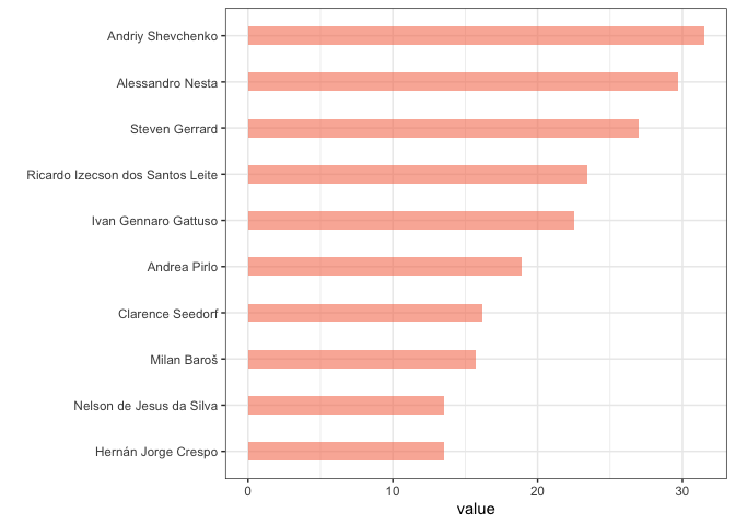we can see that the market value of Milan’s starting XI is significantly higher than Liverpool’s. Individually, Milan’s players took 8 places out of the top 10 highest market value players of the joint teams. The captain Steven Gerrard and the striker Baros are the 2 exceptions for Liverpool.

After setting the stage, let us go to the actual match.

The Data

Description

The dataset comes from the open-source github repository of the soccer data analytic company statsbomb. They make public 878 datasets in JSON format, one per game, including this one. Every dataset contains thousands of events, each event is characterized by about 100 or more variables that describe the event.

dim(istanbul)

## [1] 4648  126

The dataset that records events about the miracle of Istanbul has 4648 events, each is described by 126 variables.

head(colnames(istanbul), n = 10)

##  [1] "id"             "index"          "period"         "timestamp"     
##  [5] "minute"         "second"         "possession"     "duration"      
##  [9] "related_events" "location"

The above shows the first 10 variables. The first variable id is the unique identifier of each event; period denotes which time period this event occurs (eg. 1 = the first half); timestamp records the exact time of each event; location is another important variable that records the coordinate information of the event. An example event therefore would be: player x at time 00:31:52.716 passes the ball at the pitch coordinate (24, 40) at mid-height with angle y…. As I go forward, we will use and visualize more interesting variables.

Characteristics of the data

The dataset is really sparse (lots of NULL or NA values). This makes sense, because at one time point only one player is able to make one action. For example, Variable dribble_nutmeg is not NA if and only if some player nutmugs someone else (ouch!).

length(which(!is.na(istanbul$dribble.nutmeg)))

## [1] 4

4 nutmegs in 120 minutes (90 mins regular time plus 30 mins extra), not bad!

We need to take special care of the location variable. The location denotes the pitch coordinates of each event. The coordinate is standardized as dimension 120 * 80. However, soccer pitch size varies and the Atatürk Olympic Stadium has dimension 105 meters * 68 meters. We need to scale the coordinate from the relative location to the actual meters, so that the event will show up on the correct location on the pitch I draw.

location.x <- location.y <- rep(NA, nrow(istanbul))
for (i in 1:nrow(istanbul)) {
  if (! is.null(istanbul$location[[i]])) {
    location.x[i] <- istanbul$location[[i]][1] * 105 / 120
    location.y[i] <- istanbul$location[[i]][2] * 68 / 80
  }
}
istanbul$location.x <- location.x
istanbul$location.y <- location.y

Timeline of the match

To figure out how the game evolves, we need to know the milestones of the match. The milestones of a match are the key events, and according to convention, including match start, goals, 1st half ends, 2nd half starts, cards, substitution, penalties.

# get the goals and penalties  
goalEvents <- istanbul[which(istanbul$shot.outcome.id == 97 | istanbul$shot.type.name == "Penalty"), ]
# get the subs
subEvents <- istanbul[which(!is.na(istanbul$substitution.outcome.name)), ]
# get the cards 
cardEvents <- istanbul[which(!is.na(istanbul$foul_committed.card.name)), ]
keyEvents <- rbind(goalEvents, subEvents, cardEvents)
# Format the data to conform to timevis 
contents <- c("First half", "Second half", "1st half extra", "2nd half extra", "Penalty shootout")
contents <- c(contents, "yellow card", "yellow card")
contents <- c(contents, "Kewell out, Smicer in", "Finnan out, Hamann in", "3-1", "3-2", " 3-3", "Baros out, Cisse in", "O","O", "X","O")
contents <- c(contents, "1-0", "2-0", "3-0", "Crespo out, Tomasson in", "Seedorf out, Serginho in", "Gattuso out, Rui Costa in", "X",  "X", "O",  "O",  "X")
contents <- c(contents, "Timeout")
start <- c("2005-5-25 19:45:00", "2005-5-25 20:45:00", "2005-5-25 21:30:00", "2005-5-25 21:45:00", "2005-5-25 22:00:00")
# liverpool
start <- c (start, "2005-5-25 21:15:28", "2005-5-25 21:19:58"
, "2005-5-25 20:07:00", "2005-5-25 20:45:00", "2005-5-25 20:53:04", "2005-5-25 20:55:02", "2005-5-25 20:59:52", "2005-5-25 21:24:28", "2005-5-25 22:00:50", "2005-5-25 22:02:37", "2005-5-25 22:04:11", "2005-5-25 22:05:44")
# Milan
start <- c(start, "2005-5-25 19:45:51", "2005-5-25 20:23:12", "2005-5-25 20:27:57", "2005-5-25 21:24:50", "2005-5-25 21:25:05", "2005-5-25 21:51:20", "2005-5-25 22:00:02", "2005-5-25 22:01:40", "2005-5-25 22:03:17", "2005-5-25 22:05:03", "2005-5-25 22:06:24")
start <- c(start, "2005-5-25 20:30:00")
end <- c("2005-5-25 20:30:00", "2005-5-25 21:30:00", "2005-5-25 21:45:00", "2005-5-25 22:00:00", "2005-5-25 22:07:00", rep(NA, 23), "2005-5-25 20:45:00")
group = c(rep("time", 5), rep("Liverpool", 12), rep("Milan", 11), NA)
style = c(rep(NA, 5), rep("color:yellow;",2), rep(NA, 8), "color:red;", NA, rep(NA, 6), rep("color:red;",2), NA, NA, "color:red;", NA)
data = data.frame(content=contents, start, end, group, style)

timevisDataGroups <- data.frame(
  id = c("time", "Liverpool", "Milan"),
  content = c("Time", "Liverpool", "Milan")
)
library(timevis)
timevis(data, groups = timevisDataGroups)

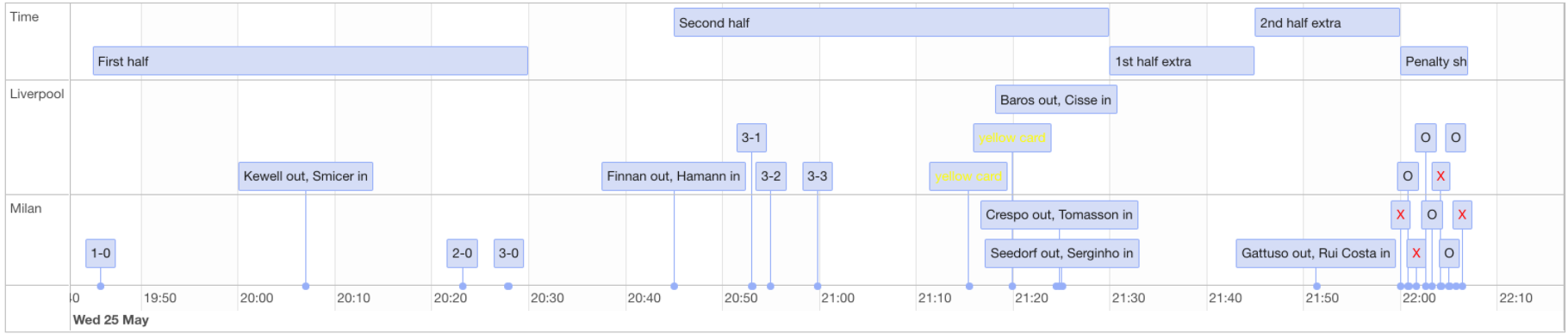
To summarize the timeline that we see above. In the first half, Milan scored immediately when the game began, and scored two more goals towards the end of the first half. On the other hand, Liverpool made a substitute because of injury. Before the start of the 2nd half, Liverpool was already 3-0 down and used one (out of total 3) substitution involuntarily. At the beginning of the 2nd half, Liverpool made yet another substitution. This substitution is due to the tactical consideration by the Liverpool manager, trying to turn things around, and it did. About 10 minutes later, Liverpool score their first goal, making it 3-1, and in this 6 minutes spell, they score three goals in total, levelling the score to 3-3. Both teams did not score in the later parts of the game, and Liverpool beat Milan 3-2 in Penalty shootout (the red X denotes penalty missing or being saved by the goalkeeper).

By seeing this timeline plot, all the key events are laid out clearly. Furthermore, we can immediately gain insights towards our question, which is, how the miracle happened:

The three comeback goals were scored in 6 minutes! What happened in those 6 minutes?
The distribution of goals are quite “even”, in that Milan scored 3 in the first half and Liverpool scored 3 in the second half. Why that is the case?

Another thing that stands out from the timeline graph is that there were only 2 yellow cards (all from Liverpool) and 0 red card in the game. That is extremely rare for a soccer game, especially for the Champions League final, the biggest game of the year. It shows how both teams were focusing on playing the game actively, not on playing the game passively (by fouling a lot to stop the other team’s play). It is truly a smooth and high quality game, and dramatic.

Heaven or Hell

As the timeline suggested, we see a distinction between the 1st half and the 2nd half. Each team scored three goals and the other team scored nothing. Specifically, the 1st half is the heaven for Milan, the hell for Liverpool; the 2nd half is exactly the reverse of the 1st half. Can we visualize the difference, the difference between heaven and hell?

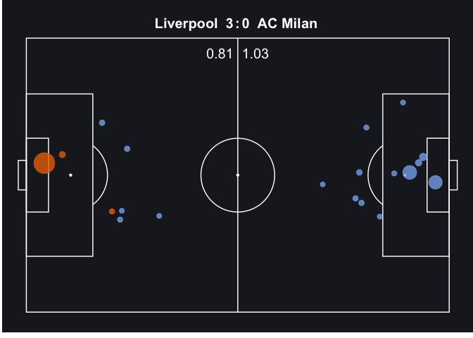
Shots

is <- tibble::as_tibble(istanbul)
is %>%
  filter(minute < 46) %>%
  soccerShotmap(theme = "dark")

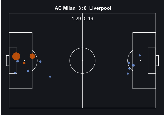
As we can see, in the 1st half, Milan made 8 shots (8 dots on the pic above) and Liverpool made 5. However, most of the shots by Milan (6 out of 8) were inside the box, whereas Liverpool only had 2.

is %>%
  filter(minute >= 45 & minute <= 90) %>%
  soccerShotmap(theme = "dark")

In the 2nd half, we’d expect that Liverpool dominates the shots and shots in the box. On the contrary, Milan still dominates the number of shots and shots in the box. Liverpool made only 2 shots inside the box and they all made it into the net, and Liverpool also scored a long-ranger. However, Milan attempted 6 shots inside the box and 6 more outside the box, none of them made it.

Let’s see the comparison between shots made by both teams in the extra time.

is %>%
  filter(minute >= 90 & minute <= 120) %>%
  soccerShotmap(theme = "dark")

Surprisingly (or not so surprisingly after seeing the shots made in the 2nd half of the game), Liverpool made no attempts and Milan made 7 more shots, 3 of them inside the box with 1 near the post of the goal (so close!) and yet, Milan scored nothing.

Passes

Passes are a essential part of a soccer game. By looking at the locations of the passes (both the starting locations and the end locations), we can also see the positions of the ball and the players.

1st half

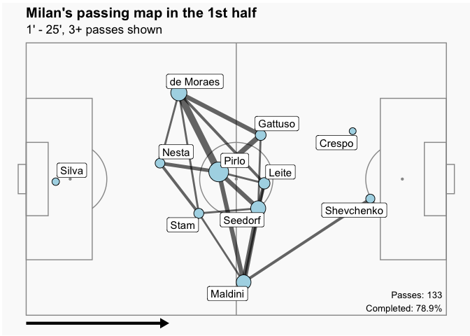
is %>%
  filter(team.name == "AC Milan" & period == 1 & minute <= 24) %>%
  soccerPassmap(fill = "lightblue", arrow = "r",
                title = "Milan's passing map in the 1st half")

picture 1

is %>%
  filter(team.name == "AC Milan" & period == 1 & minute > 24) %>%
  soccerPassmap(fill = "lightblue", arrow = "r",
                title = "Milan's passing map in the 1st half (25' onwards)")

picture 2

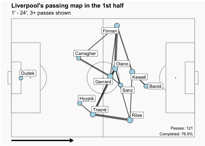
is %>%
  filter(team.name == "Liverpool" & minute <= 24 & period == 1) %>%
  soccerPassmap(fill = "lightblue", arrow = "r",
                title = "Liverpool's passing map in the 1st half")

picture 3

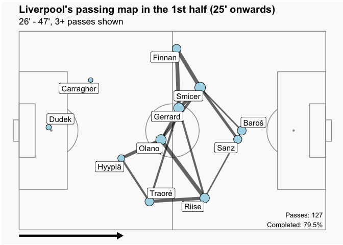
is %>%
  filter(team.name == "Liverpool" & minute > 24 & period == 1) %>%
  soccerPassmap(fill = "lightblue", arrow = "r",
                title = "Liverpool's passing map in the 1st half (25' onwards)")

picture 4

We break the 1st half into two halves. The picture 1 shows the passing map of AC Milan in the first 24 minutes, with Pirlo being the center of the passing map (the biggest blue dot in the map), Milan’s transition (from attack to defense and vice versa) depended on him. Another thing to notice is that one of the Milan’s forward, Crespo, was not really involved in the game. The picture 2 is the passing map of Milan in the second half of the 1st half. Compared to the first picture, Milan’s formation retrieved to their goal. For example, in the first 24 minutes, Maldini (left back), Gattuso, Seedorf, were standing in front of the Pirlo; they were behind Pirlo in the later half of the 1st half. I would guess the reason was due to the increase in aggressiveness of Liverpool, as well as their own strategy of contracting their defensive lines and playing counterattack, since they led 1-0 as early as 1 minute into the game. And that strategy was fantastic! They scored two more goals on counter attack at 39’ and 44’ when Liverpool tried really hard attacking (since they were 1-0 behind). The scorer of both goals is Crespo, the man who were not “involved” in terms of passing in the first 24 minutes, and he became lethal in the second part.

The picture 3 and 4 tell the Liverpool’s part of the story in the 1st half. The first thing to notice is that Kewell was out and Smicer was in for him (Kewell was in the 3rd pic but not in the 4th, and Smicer the opposite) because Kewell was injured. And compared the 4th with the 3rd picture, Gerrard and Sanz were pushing forward and to the center, while the two wingers Riise and Smicer were roughly in the same position as before.

The six minute spell

is %>%
  filter(team.name == "AC Milan" & minute >= 53 & minute <= 60) %>%
  soccerPassmap(fill = "lightblue", arrow = "r",
                title = "Milan's passing map in the 6 minute spell", minPass = 1)

picture 1

passMap(is, "AC Milan", 2, 54, 60)

picture 2

is %>%
  filter(team.name == "Liverpool" & minute >= 53 & minute <=60) %>%
  soccerPassmap(fill = "lightblue", arrow = "r",
                title = "Liverpool's passing map in the 6 minute spell", minPass = 1)

picture 3

passMap(is, "Liverpool", 2, 54, 60)

picture 4

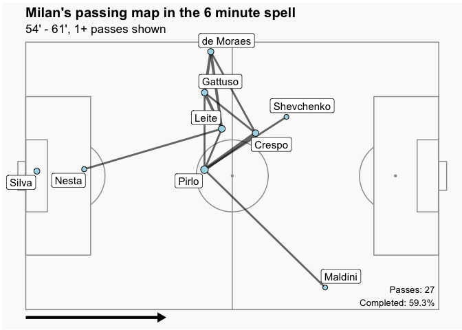
We have seen the hell for Liverpool, i.e., the first half of the game, where Milan scored an early goal and player on counter and scored two more goals while Liverpool was struggling in attacking. However, as the timeline suggests, in the second half of the game, there was a 6-minute spell where Liverpool scored 3 goals. That spell was really the heaven for Liverpool and for Liverpool’s fans. What happened? Since we are in the passing section and analyzing passes are really effective in analyzing the whole game, let’s look at all the passes happened in that spell. In the picture 1, Milan achieved 27 passes with less than 60% of them completed. Only 8 players of Milan were involved in passing the ball one or more times. Looking more closely, the picture 2 indicated that the passes from defense to midfield and midfield to attack all failed (red: failure, blue: success).

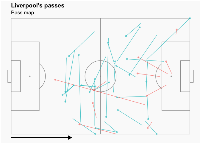
On the contrary, the picture 3 shows that all 10 players (excluding the goalkeeper) were involved in passing, and they achieved more than 75% passing accuracy. The picture 4 shows the exact passes.

In the 1st half, the passing accuracy was 78% for Milan. What causes this decline in passing accuracy and number of passes on the Milan side, whereas Liverpool somehow maintained their passing accuracy? I then look at the defensive acts by both teams in that six minutes.

d2 <- is %>% 
  filter(type.name %in% c("Interception", "Block", "Dispossessed", "Ball Recovery") & team.name == "Liverpool" & period == 2 & minute >= 54 & minute <= 60)

soccerPitch(arrow = "r", 
            title = "Liverpool", 
            subtitle = "Defensive actions") +
  geom_point(data = d2, aes(x = location.x, y = location.y, col = type.name), size = 3, alpha = 0.5)

picture 1

d2 <- is %>% 
  filter(type.name %in% c( "Interception", "Block", "Dispossessed", "Ball Recovery") & team.name == "AC Milan" & period == 2 & minute >= 54 & minute <= 60)

soccerPitch(arrow = "r", 
            title = "Milan", 
            subtitle = "Defensive actions") +
  geom_point(data = d2, aes(x = location.x, y = location.y, col = type.name), size = 3, alpha = 0.5)

picture 2

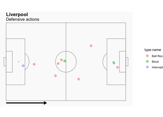
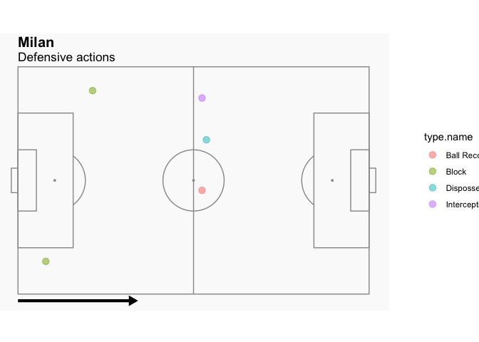
The picture 1 is the defensive actions done by Liverpool players in 6 minutes. What is staggering is that they managed to achieve 7 ball retrievals, leading to the decline in Milan’s passing accuracy. The picture 2 shows the defensive actions done by Milan. The mere 1 ball retrieve hardly influenced Liverpool’s passing and possession.

Position

We have seen some visual information about the position of the players in the passing maps earlier, to the point that we saw some deliberate position shifts from the Milan side in the 1st half when they contracted their defense lines. Through the viualizations below, we can see more about the shifts in positions in terms of the whole team (i.e. shifts in team formation) and individual key players.

1st half

is %>%
  filter(!is.na(location.x) & team.name == "AC Milan" & period == 1) %>% 
  soccerPositionMap(id = "player.name", x = "location.x", y = "location.y", 
                    fill1 = "blue", theme = "grass", arrow = "r", 
                    title = "AC Milan", 
                    subtitle = "Average position (1st half)")

picture 1

is %>%
  filter(!is.na(location.x) & team.name == "Liverpool" & period == 1 & minute >= 25) %>% 
  soccerPositionMap(id = "player.name", x = "location.x", y = "location.y", 
                    fill1 = "blue", theme = "grass", arrow = "r", 
                    title = "Liverpool", 
                    subtitle = "Average position (1st half)")

picture 2

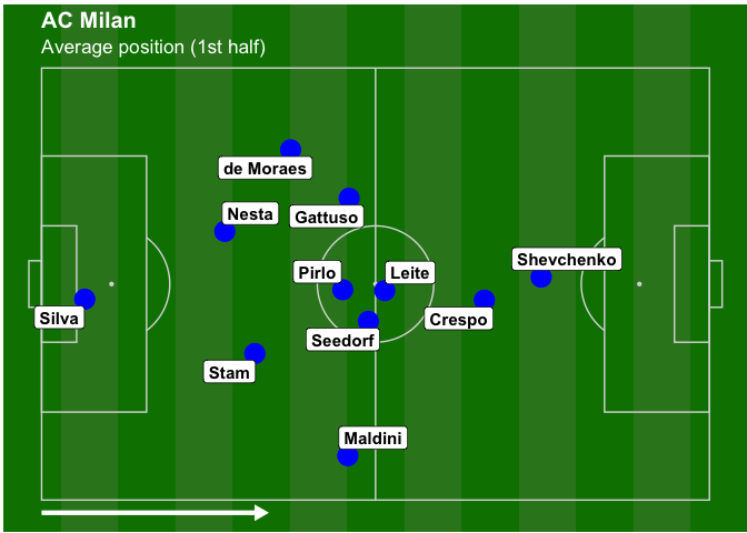
The picture 1 is the average position of the Milan in the 1st half. The average position is defined as the average coordinates of players when they take any actions, not only the passing ones. As we can see, the Milan’s formation were really tight in the center of the midfield. In addition to the 4 midfielders, one of the forwards Crespo was close to midfield as well. And they were close together in the center for a reason (as explained below).

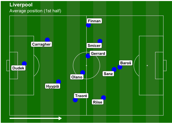
In the picture 2, Liverpool’s formation in the 1st half was rather scattered acrossthe width of the field. This was due to their tactics of playing wide on the sides. Gerrard and Olano were together as a pair, sitting in the midfield. However, their attacks on the sides were not going very well, so Milan decided not to put too many players on the sides (indicated by the 1st pic) and focused their attacks and later their counter attacks in the center.

first 15 mins at 2nd half

is %>% 
  filter(!is.na(location.x) & team.name == "AC Milan" & period == 2 & minute <= 60) %>% 
  soccerPositionMap(id = "player.name", x = "location.x", y = "location.y", 
                    fill1 = "blue", theme = "grass", arrow = "r", 
                    title = "AC Milan", 
                    subtitle = "Average position (2nd half)")

picture 1

is %>%
  filter(!is.na(location.x) & team.name == "Liverpool" & period == 2 & minute <= 60) %>% 
  soccerPositionMap(id = "player.name", x = "location.x", y = "location.y", 
                    fill1 = "blue", theme = "grass", arrow = "r", 
                    title = "Liverpool", 
                    subtitle = "Average position (2nd half)")

picture 2

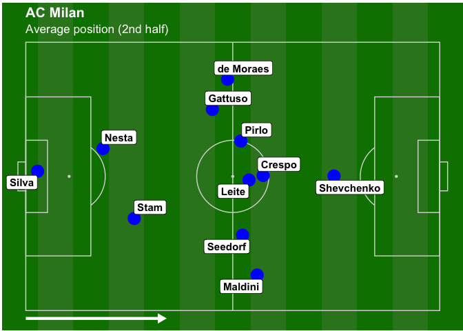
With 3-0 down, Liverpool took right back Finnan down (therefore forfeiting the attacking on the sides tactics) and put Hamman up immediately in the beginning of the 2nd half, and the result was astonishing! In the picture 2, Hamann took the position of where Gerrard was in the 1st half, and freed Gerrard. By sacrificing the right back, the Liverpool squeezed their formation towards the center. Gerrard, together with Sanz and Baros, were constantly charging to the Milan’s box carefree, since Hamann took care of his defensive duties. And Boom! Gerrard scored the first goal, a header inside the box, and created a penalty (later converted to the 3rd goal).

Conclusion

Some may say that there is no need to visualize a soccer match, since it is a visual art/sport in itself. I have to agree since I am a soccer fan and have had so much joy and pain watching the games. It is especially hard to try to visualize a miracle. However, I did it anyway because an EDA process on a soccer match dataset can achieve the following things:

A visual summary. In normal games, audiences see the motions of players in terms of motions of pictures, and they do not have good enough memory to remember everything and do not have time to summarize those information, as they are concentrated on the game itself. After the match, audiences will see lots of statistics about the game, such as the number of shots, the possession rate, number of passes, pass accuracy, etc, and they do not make much sense and they are not even comparable. A 65% possession rate in a game by a side is not the same thing as another team having 65% in another game. Go ask Barcelona fans. Their team used to have 65% possession and ended up winning all trophies, and now win nothing with the same possession rate. Visualizations like this can combine the visual part with the summary part, providing fans with a more immersive and insightful perspective towards understanding the game.
A good starting point for models about soccer game. As the advance of data science, models about soccer games are in dire need. A prominent example would be the model to predict expected goals given the data about soccer games. This EDA process is great for:
1. See the data and find the characteristics of the data. In my example, it would be a lot of None values in the dataset and incompatible field dimension that I need to manually change.
2. Visualize the key events that may lead to goals.
3. Find out directions that may worth pursuing. I find out the 6 minute Liverpool spell and think this may be the direction to look further into.

Main lessons learnt: It is no doubt a miracle, because:

Super dramatic. Liverpool dominated the game for only 6 minutes, and ended up scoring three goals. Milan took the show for 114 minutes, including 7 shots in extra time, and they failed to score any after the 1st half. The inefficiency in shooting influenced their mindset in the final penality shoot out, missing 3 out of 5. And Dudek’s (Liverpool’s goalkeeper) double save from Shevchenko in the 117th minute was voted the greatest Champions League moment of all time.
Some reasons behind the comeback drama. 6 minutes spell because of the introduce of Hamann that freed Gerrard to attack. Milan’s success in the 1st half was also due to the formation factor, where Milan was tight in the center and Liverpool scattered.
Human factor. The hard part to visualize. The psychological change of the Milan side as they went from ecstasy to doubt, and to fear. Their change in mindset when they repeatedly attack but scored nothing. On the other side, Gerrard and his influence on the whole team.

Credits

Data

Statsbomb

Visualization package

soccermatics
ggplot2

My working session

sessionInfo()

## R version 4.1.0 (2021-05-18)
## Platform: x86_64-apple-darwin20.4.0 (64-bit)
## Running under: macOS Big Sur 11.4
## 
## Matrix products: default
## BLAS:   /usr/local/Cellar/openblas/0.3.15_1/lib/libopenblasp-r0.3.15.dylib
## LAPACK: /usr/local/Cellar/r/4.1.0/lib/R/lib/libRlapack.dylib
## 
## locale:
## [1] en_US.UTF-8/en_US.UTF-8/en_US.UTF-8/C/en_US.UTF-8/en_US.UTF-8
## 
## attached base packages:
## [1] parallel  stats     graphics  grDevices utils     datasets  methods  
## [8] base     
## 
## other attached packages:
##  [1] forcats_0.5.1      RColorBrewer_1.1-2 soccermatics_0.9.4 StatsBombR_0.1.0  
##  [5] tidyr_1.1.3        sp_1.4-5           purrr_0.3.4        jsonlite_1.7.2    
##  [9] httr_1.4.2         doParallel_1.0.16  iterators_1.0.13   foreach_1.5.1     
## [13] RCurl_1.98-1.3     rvest_1.0.0        tibble_3.1.2       stringr_1.4.0     
## [17] stringi_1.6.2      dplyr_1.0.6        ggplot2_3.3.3     
## 
## loaded via a namespace (and not attached):
##  [1] zoo_1.8-9         tidyselect_1.1.1  xfun_0.23         lattice_0.20-44  
##  [5] colorspace_2.0-1  vctrs_0.3.8       generics_0.1.0    htmltools_0.5.1.1
##  [9] yaml_2.2.1        utf8_1.2.1        rlang_0.4.11      R.oo_1.24.0      
## [13] pillar_1.6.1      glue_1.4.2        withr_2.4.2       R.utils_2.10.1   
## [17] tweenr_1.0.2      plyr_1.8.6        lifecycle_1.0.0   munsell_0.5.0    
## [21] gtable_0.3.0      SDMTools_1.1-221  R.methodsS3_1.8.1 codetools_0.2-18 
## [25] evaluate_0.14     knitr_1.33        fansi_0.5.0       xts_0.12.1       
## [29] Rcpp_1.0.6        scales_1.1.1      farver_2.1.0      ggforce_0.3.3    
## [33] digest_0.6.27     ggrepel_0.9.1     polyclip_1.10-0   grid_4.1.0       
## [37] cowplot_1.1.1     tools_4.1.0       bitops_1.0-7      magrittr_2.0.1   
## [41] crayon_1.4.1      pkgconfig_2.0.3   ellipsis_0.3.2    MASS_7.3-54      
## [45] xml2_1.3.2        rmarkdown_2.8     R6_2.5.0          compiler_4.1.0

source code

code

Introduction#

The underdog#

The Data#

Description#

Characteristics of the data#

Timeline of the match#

Heaven or Hell#

Shots#

Passes#

1st half#

The six minute spell#

Position#

1st half#

first 15 mins at 2nd half#

Conclusion#

Credits#

Data#

Visualization package#

My working session#

source code#

Introduction

The underdog

The Data

Description

Characteristics of the data

Timeline of the match

Heaven or Hell

Shots

Passes

1st half

The six minute spell

Position

1st half

first 15 mins at 2nd half

Conclusion

Credits

Data

Visualization package

My working session

source code